This new applet is designed for students to practise conversion of common units used in physics on their own. There is a checking algorithm within, which might need some fine-tuning. For full screen view, click here.
The worked solutions given will demonstrate the breakdown of steps that could help students learn the procedure to convert these units.
This little applet is designed to allow students to change the order of magnitude and to use any common prefix to observe how the physical quantities are being written. To view this applet in a new tab, click here.
Standard form (also known as scientific notation) is a way of writing very large or very small numbers that allows for easy comparison of their magnitude by using the powers of ten. Any number that can be expressed as a number, between 1 and 10, multiplied by a power of 10, is said to be in standard form.
For instance, the speed of light in vacuum can be written as 3.00 × 10⁸ m s–1 in standard form.
When a prefix is added to a unit, the unit is multiplied by a numerical value represented by the prefix. e.g. distance = 180 cm = 180 x 10-2 m = 1.80 m
The purpose of using prefixes is to reduce the number of digits used in the expression of values. Hence, students can use the prefix slider to find a user-friendly expression, such as 682 nm instead of 0.000000682 m.
This rather informative video uses a recent local case of electrocution as a case study and goes on to explain various practical electricity concepts such as electric faults (e.g. live wire connected to earth wire). Recommended for students learning about O-level Practical Electricity, although I would caution them that some of the dialogue is based on a layman’s understanding of how electricity works, so there are some scientific inaccuracies.
This interactive is designed to help students understand the statistical approach underpinning the drawing of a best-fit line for practical work. For context, our national exams have a practical component where students will need to plot their data, often following a linear trend, on graph paper and to draw a best-fit line to determine the gradient and y-intercept.
The instructions to students on how to draw the best-fit line is often procedural without helping students understand the principles behind it. For instance, students are often told to minimise and balance the separation of plots from the best-fit line. However, if there are one or two points that are further from the rest from the best-fit line (but not quite anomalous points that need to be disregarded), students would often neglect that point in an attempt to bring the best fit line as close to the remaining points as possible. This results in a drastic increase in the variance as the differences are squared in order to calculate the “the smallest sum of squares of errors”.
This applet allows students to visualise the changes in the squares, along with the numerical representation of the sum of squares in order to practise “drawing” the best-fit line using a pair of movable dots. A check on how well they have “drawn” the line can be through a comparison with the actual one.
Students can also rearrange the 6 data points to fit any distribution that they have seen before, or teachers can copy and modify the applet in order to provide multiple examples of distribution of points.
There is a new internet trend called “tensegrity” – an amalgamation of the words tension and integrity. It is basically a trend of videos showing how objects appear to float above a structure while experiencing tensions that appear to pull parts of the floating object downwards.
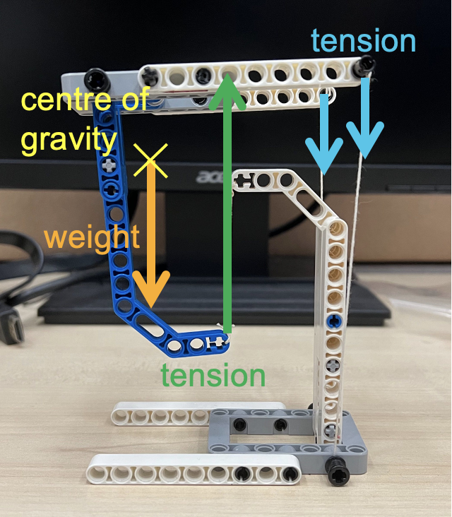
In the diagram below, the red vectors show the tensions acting on the “floating” object while the green vector shows the weight of the object.
The main force that makes this possible is the upward tension (shown below) exerted by the string from which the lowest point of the object is suspended. The other tensions are downward and serve to balance the moment created by the weight of the object. The centre of gravity of the “floating” structure lies just in front of the supporting string. The two smaller downward vectors at the back due to the strings balance the moment due to the weight, and give the structure stability sideways.
This is a fun demonstration to teach the principle of moments, and concepts of equilibrium.
The next image labels the forces acting on the upper structure. Notice that the centre of gravity lies somewhere in empty space due to its shape.
Only the forces acting on the upper half of the structure are drawn in this image to illustrate why it is able to remain in equilibrium
These tensegrity structures are very easy to build if you understand the physics behind them. Some tips on building such structures:
Make the two strings exerting the downward tensions are easy to adjust by using technic pins to stick them into bricks with holes. You can simply pull to release more string in order to achieve the right balance.
The two strings should be sufficiently far apart to prevent the floating structure from tilting too easily to the side.
The centre of gravity of the floating structure must be in front of the string exerting the upward tension.
The base must be wide enough to provide some stability so that the whole structure does not topple.
Here’s another tensegrity structure that I built: this time, with a Lego construction theme.
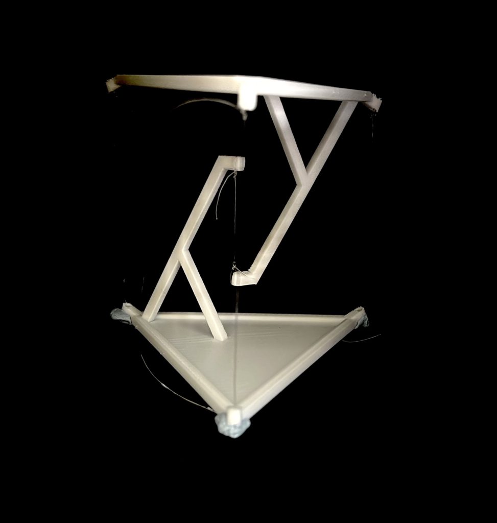
Apart from using Lego, I have also 3D-printed a tensegrity structure that only requires rubber bands to hold up. In this case, the centre of gravity of the upper structure is somewhere more central with respect to the base structure. Hence, 3 rubber bands of almost equal tension will be used to provide the balance. The STL file for the 3D model can be downloaded from Thingiverse.com.
The main challenge in assembling a tensegrity structure is the adjustment of the tensions such that the upper structure is balanced. One way to simplify that, for beginners, is to use one that is supported by rubber bands as the rubber bands can adjust their lengths according to the tensions required.
3D-printed tensegrity table balanced by rubber bands
Another tip is to use some blu-tack instead of tying the knots dead such as in the photo below. This is a 3D printed structure, also from Thingiverse.
3D-printed tensegrity table held up and balanced by nylon string
(This post was first published on 18 April 2020 and is revised on 24 August 2022.)
Came across a question recently that many students answered incorrectly.
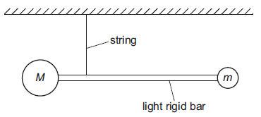
Close to the surface of the Earth the gravitational field strength is uniform. A pair of unequal masses are joined by a light, rigid horizontal bar and suspended by a string from their centre of gravity as shown. The mass M of the ball on the left is larger than the mass m of the ball on the right.
The supporting string is now cut and the system begins to fall. Air resistance is negligible.
Which statement is correct?
A
The bar will remain horizontal as it falls.
B
The bar will rotate clockwise as it falls.
C
The bar will rotate anti-clockwise as it falls.
D
The bar will first rotate clockwise and then rotate anticlockwise as it falls.
Without air resistance
This question supposes that air resistance is negligible and so the only forces initially acting on the object is weight. The answer that many students gave incorrectly as B because they assume that the larger weight acting on the larger mass will bring about a larger acceleration.
Since the object begins in equilibrium, and the acceleration of both objects is just gravitational acceleration, the bar will remain horizontal.
With air resistance
This then invites a question: What if there is air resistance?
To consider the vertical acceleration on both balls, we need to consider the net force $F_{net}$, which is the vector sum of weight $W$ and air resistance $F_R$, ignoring the tension exerted by the rod at the initial stage of the fall.
$$F_{net} = W – F_R = V \rho_{ball}g – \dfrac{1}{2} \rho_{air}v^2C_DA$$
The volume V of a sphere is proportional to $r^3$ and its cross-sectional area A is proportional to $r^2$,
A larger radius will imply a larger increase in V than A, and hence, a large $W$ than $F_R$. This will then allow the larger mass to experience a larger acceleration than the smaller mass in the initial stage.