I added a check for the text input so that users have to key in the correct number of decimal places according to the precision of the instrument. For instance, a reading of 1 V should be recorded as 1.00 V and 1.5 V recorded as 1.50 V. Users need to read to half the smallest division, e.g. if the needle is between 2.4 and 2.5, they should input 2.45 V.
As evidence of the prowess of generative AI, this graph plotting app was created in about 15 minutes with simple prompts and a text editor. It was tested with an existing set of data and uploaded immediately to the repository.
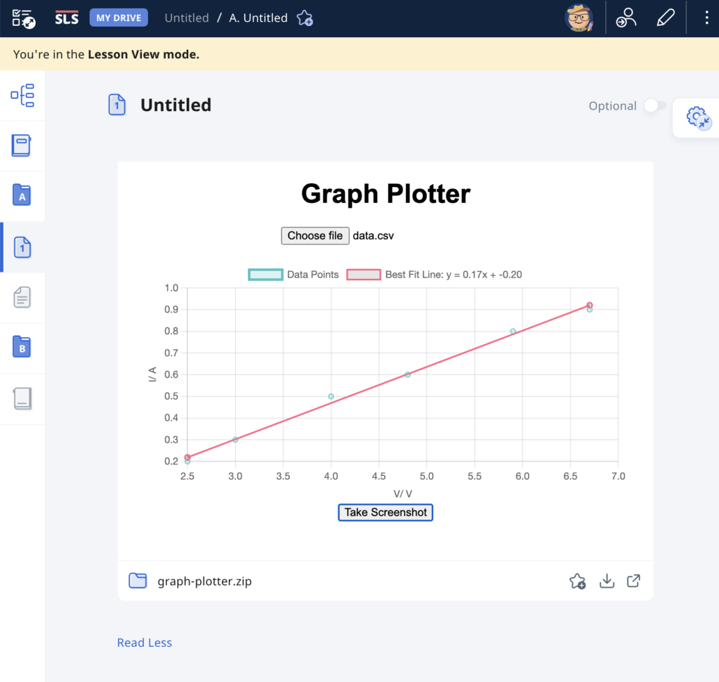
The user will begin by uploading a set of data from an experiment, with the column header being the labels for the axes, in the form of a CSV file. The app immediately calculates and displays the best-fit straight line using linear regression, providing users with insights into the relationships between the variables in the dataset. This allows for easy analysis of trends, patterns, and relationships within the data. Students can use the app to quickly visualize and analyze data. The screenshot button enables them to save the graph in picture form for submission to their teachers.
It has also been made compatible with the Student Learning Space. The screenshots saved by students can be uploaded as an attachment for a free-response question. This is especially useful when students are doing lab work and the teacher does not want the students to bother too much with configuring the graph. The ZIP file for use in the SLS can be downloaded here.
Prompts used are:
Create a website using html and javascript for users to plot a graph using data from a csv file.
The user can upload a csv file with the first column being the horizontal axis and the second column being the vertical axis.
The column headers, which is the first set of values in the csv file, will form the labels for the axes of the graph.
Plot the points with the data in the csv file and use linear regression to obtain the best-fit straight line of the data.
The best fit line should be a line joining two red dots.
Indicate the gradient and intercept of the best-fit line.
Add a button at the bottom for users to take a screenshot of the graph.
This interactive is designed to help students understand the statistical approach underpinning the drawing of a best-fit line for practical work. For context, our national exams have a practical component where students will need to plot their data, often following a linear trend, on graph paper and to draw a best-fit line to determine the gradient and y-intercept.
The instructions to students on how to draw the best-fit line is often procedural without helping students understand the principles behind it. For instance, students are often told to minimise and balance the separation of plots from the best-fit line. However, if there are one or two points that are further from the rest from the best-fit line (but not quite anomalous points that need to be disregarded), students would often neglect that point in an attempt to bring the best fit line as close to the remaining points as possible. This results in a drastic increase in the variance as the differences are squared in order to calculate the “the smallest sum of squares of errors”.
This applet allows students to visualise the changes in the squares, along with the numerical representation of the sum of squares in order to practise “drawing” the best-fit line using a pair of movable dots. A check on how well they have “drawn” the line can be through a comparison with the actual one.
Students can also rearrange the 6 data points to fit any distribution that they have seen before, or teachers can copy and modify the applet in order to provide multiple examples of distribution of points.
I am taking the opportunity (since my students are all doing home-based learning) to teach them how to use spreadsheets to do calculations and to obtain a best-fit line. While they can still submit graph work using PDF scanning apps such as Office Lens and Camscanner into Google Classroom for me to mark, they can make use of the spreadsheet-generated graph to check their results.
Even though for exams, we still require them to plot the points on paper and obtain the gradient and intercept from points on the best-fit line, nobody is going to do so when they start working. So I might as well teach them now.
Due to the lack of face-to-face time, I made this step-by-step video showing them how to do so.
For lab work, students often have to estimate a line of best fit for their data points manually. It takes a bit of practice to get it right. With this app, students can generate data points with varying types of scatter and predict their own best-fit line before comparing it with a computer generated one based on the least mean square method.
The following is the script that I used for recording the video above for our e-learning day. I’m posting it here as I can edit it easily via wordpress’s mobile app, and because I have LaTeX enabled here.
Aim:
The aim of this planning question is to investigate how the resonant frequency of a wire vibrating in its fundamental mode depends on the tension in the wire.
The independent variable is the tension in the string which can be varied by hanging masses at one end of the wire and dangling that end over the edge of a table on a pulley. The tension is represented by the symbol.
The dependent variable is the resonant frequency of the fundamental mode in the wire. The fundamental mode consists of two nodes at both ends of the wire and one antinode in the middle.
In other words, in our experiment, we shall vary tension and measure the resonant frequency of the fundamental mode.
The length of wire between the supports is kept constant throughout the experiment and we shall use the same wire throughout so that the mass per unit length is kept constant.
Procedure:
The experiment will be set up according to this diagram. One end of the wire is first tied to a fixed object. The other end is hanging over a pulley clamped on the edge of the laboratory table and tied to a mass hanger. To control the length of the wire, place a bridge at each end. Only the length of the wire between the two bridges will be vibrating. We shall keep this length constant for the whole experiment.
Record the mass of the mass hanger m and determine its weight. The weight mg is taken to be equal to the tension T on the string.
A uniform horizontal magnetic field is generated by a pair of large electromagnetic coils on both sides of the wire. The wire is connected on both ends to a function generator. An alternating current is produced by the function generator and its frequency can be varied using the same apparatus. The function generator should have a display that enables us to read the frequency.
The resulting magnetic force acting on the wire will be driving the oscillation of the wire at the frequency shown on the function generator. By adjusting the frequency of the alternating current until the fundamental mode of a standing wave is formed on the wire, we can record the resonant frequency fo for the corresponding tension T.
We shall repeat the experiment for different values of m by adding known amounts of mass (e.g. 50 g increments each time) onto the mass hanger. All the values for the mass m and resonant frequency for the fundamental modes fo should be recorded and tabulated.
The tension in the wire is then calculated using the equation T = mg.
Assume that the resonant frequency for the fundamental mode fo and the tension T follows the equation fo = kTnwhere k and n are constants. Then lg fo = lg k + n lg T. Plotting a graph of lg fo versus lg T, we can conclude that the assumption is correct if a linear relationship is observed and we can obtain the values of n and k from the gradient and the vertical intercept of the graph respectively.
As a safety consideration, the person conducting the experiment should wear goggles as the wire at high tension might suddenly snap or come loose. Always handle power supply with care.
As a precaution to improve reliabiliy, we can place a white card behind the vibrating wire so it can be seen easily. To make sure that the weight of each of the slotted masses is as indicated, measure them on a weighing balance. FInally, ensure that the pulley is smooth by measuring the tension in the wire using a force meter to check that it is indeed equal to the weight of the slotted mass.