I added a check for the text input so that users have to key in the correct number of decimal places according to the precision of the instrument. For instance, a reading of 1 V should be recorded as 1.00 V and 1.5 V recorded as 1.50 V. Users need to read to half the smallest division, e.g. if the needle is between 2.4 and 2.5, they should input 2.45 V.
I used ChatGPT to create this simple interactive graph. Including the time taken to make 2 rounds of refinement using more prompts and the time it took to deploy it via Github, it took about 15 minutes from start to end.
The first prompt I used was :
Create a graph using chart.js with vertical axis being “displacement / m” and horizontal axis being “time / s”. There should be a slider for the initial velocity value ranging from 0 to 2 m/s, a slider for the acceleration value ranging from -2 m/s^2 to 2 m/s^2. The displacement will start from zero and will follow a function dependent on the initial velocity and acceleration values from the slider. Draw the line of the displacement on the graph. Update the graph whenever the sliders are moved.
The results of the first attempt is shown above. It is already functional, with the initial velocity and acceleration sliders working together to change the shape of the graph.
The function it used to calculate displacement is based on the kinematics equation $s = ut + \dfrac{1}{2}at^2$, written as
displacement.push(0.5 * acceleration * t * t + initialVelocity * t);
After the first successful attempt, I gave some refinement prompts like:
Show the values of the velocity and acceleration, along with the units.
Use drop-down list to change the vertical axis to velocity or acceleration, updating the axis each time and the curve as well.
So the second attempt looked like this
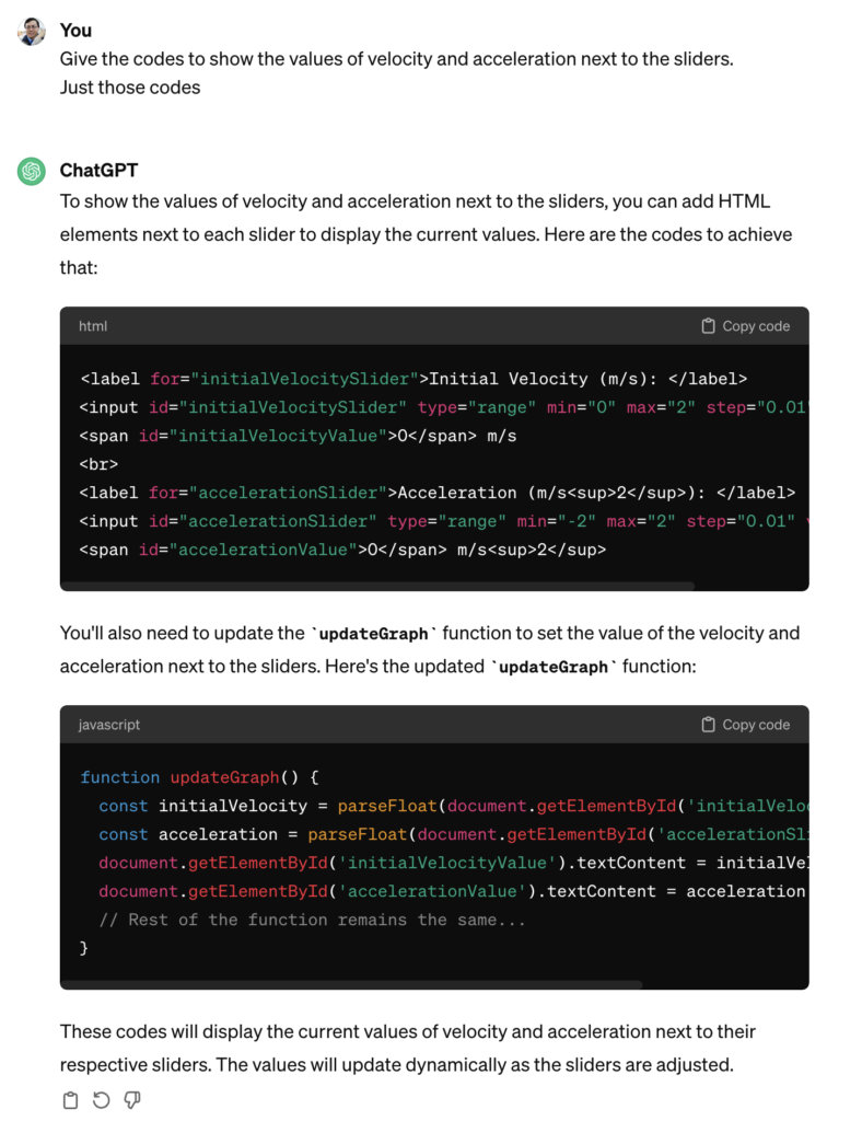
ChatGPT got 1 out of 2 requests correct. The values of the velocity and acceleration were intended to be displayed next to the sliders. It must have been because I was not clear enough. Hence, the last refinement I asked for was :
Give the codes to show the values of velocity and acceleration next to the sliders. Just those codes.
I didn’t want to get ChatGPT to generate the entire page of html and javascript again so I targetted the specific codes that I needed to change.
It was helpful in telling me where to update these codes. So at the end of the day, this is what was obtained after I made some manual tweaks to change the way the unit is displayed (e.g. m s-2 instead of m/s2):
It was good enough for my purpose now. The web app can be sent to students as a link (https://physicstjc.github.io/sls/kinematics-graph) or embedded into SLS as a standalone app. For use in SLS, do note the following:
The html file must be named index.html
The chart.js file must be copied and saved in the same zipped file at the same level as the index.html file. Change the path of the Chart JS from <script src=”https://cdnjs.cloudflare.com/ajax/libs/Chart.js/3.7.0/chart.min.js”></script> to <script src=”chart.min.js”></script>.
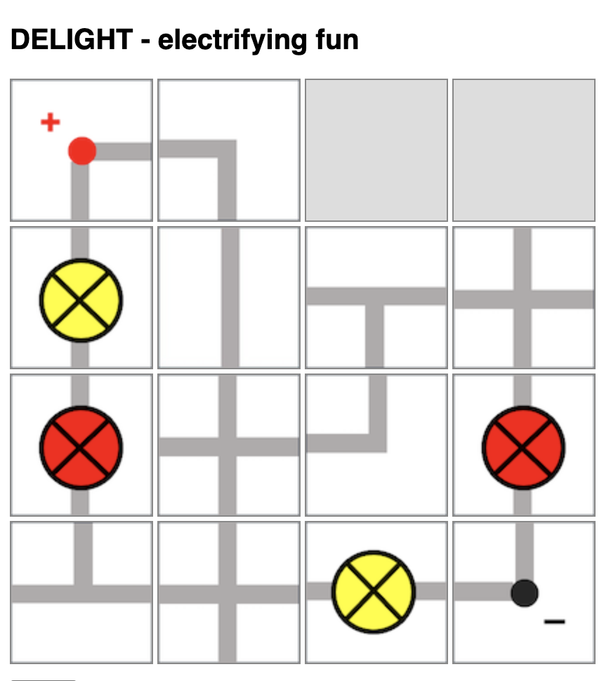
I had previously shared about this physical board game that I designed to teach electricity concepts. Now, with ChatGPT’s help, I have managed to produce a simple implementation of the board game so that there is no need to print and cut out the pieces anymore.
However, the game is still unable to detect if the light bulb will light up and automatically change the image colour or add the scores. That will require further complex programming due to the many possible outcomes for this game.
Players will take turns to connect their own bulbs to the terminals while trying to sabotage their opponent’s bulbs.
Players will take turns to place one piece on the 4-by-4 game board by clicking to select the electrical component and clicking on the square on the board to place it.
Upon placing the piece, the player can also turn that piece in any orientation (by clicking on it) within the same turn.
Players can choose to use up to two turns at any point in the game to rotate any piece that had been placed by any player.
In other words, each player has 9 turns: 7 placement turns and 2 rotation turns.
At lower levels, students can compete to see who has the most lit bulbs. However, they will need to be able to identify which light bulbs are lit. Do watch out for short-circuits.
At higher levels, students can compete to see whose light bulbs has the most total electrical power, with some calculations involved.
It took a while due to the need to adjust the equations used based on the position of the graphs, but here it is: https://www.geogebra.org/m/dfb53dps
The kinematics of a bouncing ball can be explained by considering the dynamics and forces involved in its motion. In this simulation, air resistance is assumed negligible. When a ball is dropped from a certain height and bounces off the ground, several key principles of physics come into play. Let’s break down the process step by step:
Free Fall: When the ball is released, it enters a state of free fall. During free fall, the only force acting on the ball is gravity. This force is directed downward and can be described by W = mg
W is the gravitational force. m is the mass of the ball. g is the acceleration due to gravity (approximately 9.81 m/s² near the surface of the Earth).
Impact with the Ground and Bounce: When the ball reaches the ground, it experiences a force due to the collision with the surface. This force is an example of a contact force and much larger than the gravitational force. This force depends on the elasticity of the ball and the surface it bounces off.
During the collision with the ground, the ball’s momentum changes rapidly. If the ball and the ground are both ideal elastic materials, the ball will bounce back with the same speed it had just before impact. In reality, some energy is lost during the collision, causing the bounce to be less than perfectly elastic. This simulation assumes elastic collisions.
Post-Bounce Motion: After the bounce, the ball starts moving upward. Gravity acts on it as it ascends, decelerating its motion until it reaches its peak height.
Second Descent: The ball then starts descending again, experiencing the force of gravity pulling it back down towards the ground.
This process continues with each bounce. In practice, with each bounce, some energy is lost due to the non-ideal nature of the collision and other dissipative forces like air resistance. As a result, each bounce is typically lower than the previous one until the ball eventually comes to rest. However, for simplicity, the simulation assumes no energy is lost during the collision and to dissipative forces.
An animated gif file is included here for use in powerpoint slides:
The above is a GeoGebra applet that can be customised for any energy problem. Simply make a copy of it and change the values or labels as needed. This can be integrated into either GeoGebra Classroom or Google Classroom (as a GeoGebra assignment) and the teacher can then monitor every student’s attempt at interpreting the energy changes in the problem. The teacher can also choose different extents of scaffolding, e.g. provide the initial or final states and ask students to fill in the rest.
What is an LOL Diagram?
An LOL diagram is a tool used to visualize and analyze the conservation of energy in physical systems. “LOL” does not stand for anything meaningful. Rather, they just form the shapes of the two sets of axes and the circle in between. They help clarify which objects or components are included in the energy system being considered and how energy is transferred or transformed within that system.
In LOL diagrams:
An energy system is defined as an object or a collection of objects whose energies are being tracked.
LOL diagrams consist of three parts: a L-shaped bar-chart representing the initial state, an O representing the object (or system) of interest and another L-shaped bar-chart representing the final state.
There can also be energy transferred into the system or out of the system if the system is not closed or isolated. These are represented using horizontal bars below the L axes, with arrows indicating if they are energy transferred in or out.
When performing calculations involving the initial and final energy states, the energy transferred into the system is added to the initial energy state while the energy transferred out of the system is added to the final energy state. The sums must be equal. In other words,
Initial energy stores + Energy transferred into system = Final energy stores + Energy transferred out of system
How do I use an LOL diagram?
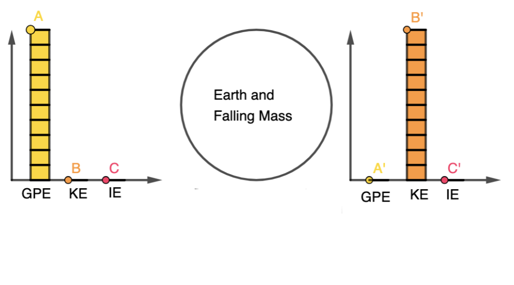
Here’s a breakdown of how LOL diagrams are used, using an example of a falling mass:
System Definition (O):
Choose what is part of the energy system (objects whose energies are being tracked) and what isn’t.
For example, in the case of a falling mass, the mass itself and the Earth are part of the energy system.
Initial State (L):
Represent the initial energy configuration of the system.
Identify the types of energy present in the system at the beginning. In this example, we begin with some gravitational potential energy.
Transition:
Show how energy changes as the system evolves. In the falling mass example, the gravitational potential energy decreases, and kinetic energy increases.
Final State (L):
Represent the energy distribution in the system at the end of the process.
In the falling mass example, at the point just before it hits the ground, kinetic energy is maximized, and gravitational potential energy is minimized.
LOL diagrams illustrate that energy within the system is conserved, meaning the total energy in the system remains constant.
External work (work done by forces outside the defined system) may impact the system’s energy, but internal work (work done within the defined system) does not change the total energy of the system.
The mathematical representation of the above problem will then simply be:
GPE = KE
$mgh = \dfrac{1}{2}mv^2$
This problem seems a bit trivial. Since LOL diagrams are a visual tool to help students and scientists analyze energy transformations and conservation, they can be used for making it easier to set up and solve conservation of energy equations in problems of greater complexity.
LOL Diagram of an Electrical Circuit
It is also important to note that the choice of the object (or system) of interest will result in different LOL diagrams for the same phenomenon.
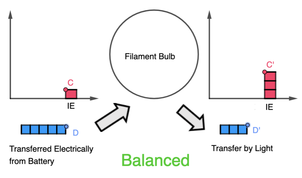
For example, consider a filament bulb in a circuit with a battery. The system at room temperature also has some energy in the internal store (or internal energy, which consists of the kinetic and potential energies of the particles in the system).
When considering the filament as the object of interest, when energy is transferred electrically from the battery, part of it is transferred by light from the bulb to the surroundings and another part is added to the internal store, as it heats up the filament light.
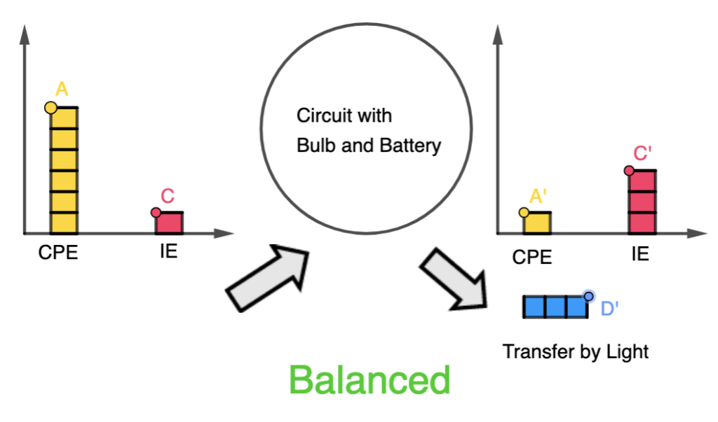
On the other hand, when considering the circuit as the whole, the chemical potential store of the battery is included in the initial energy state of the system. Hence, there is no additional energy transfer into the system but the energy transfer output is still the same.
How do I modify the GeoGebra applet to make my own LOL Diagram?
Here’s a video that demonstrates how the editing process is done, in a little more than one minute!