I modified an existing simulation to demonstrate how the displacement of particles along a longitudinal wave can be represented in graphical form. Essentially, one would have to...
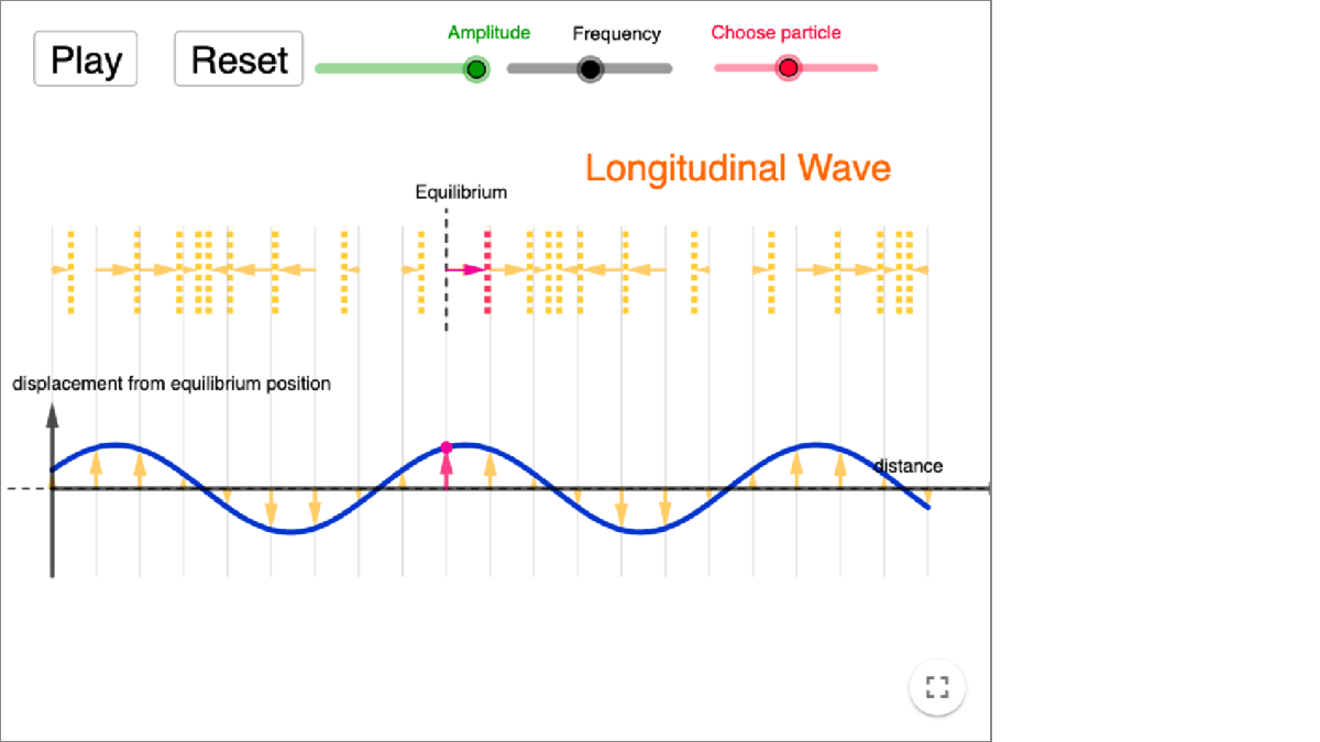
I modified an existing simulation to demonstrate how the displacement of particles along a longitudinal wave can be represented in graphical form.
Essentially, one would have to determine for each particle, its displacement from the equilibrium position and its corresponding position along the wave's direction. On the graph, positive displacement indicates movement in one direction (e.g., to the right), while negative displacement indicates movement in the opposite direction (e.g., to the left).
The commonly taught explanation (for people from my generation) for how airplanes generate lift often relies on the Bernoulli Principle, which states that faster airflow over the...
The commonly taught explanation (for people from my generation) for how airplanes generate lift often relies on the Bernoulli Principle, which states that faster airflow over the curved top of a wing reduces pressure, creating lift. However, this explanation oversimplifies the complex physics involved and is labelled an inaccurate theory by NASA. The true mechanism behind lift is better explained by the Coanda Effect, which describes how a fluid, like air, tends to follow a curved surface, such as an aerofoil.
In this video, John Collins (award winning paper airplane maker and author) explains how the Coanda Effect ensures that airflow stays attached to the wing's surface, curving around it and being deflected downward. This downward deflection of air is critical because, according to Newton's Third Law of Motion, the downward push of air results in an equal and opposite upward force—lift.
Understanding the Coanda Effect gives a more accurate picture of how lift is generated and explains why certain wing shapes and angles are more effective. Unlike the Bernoulli-based explanation, the Coanda Effect shows why airflow remains attached to the wing, ensuring the necessary conditions for lift.
Heating and cooling curves are graphical representations that show how the temperature of a substance changes as heat is added or removed over time. They illustrate the behavior...
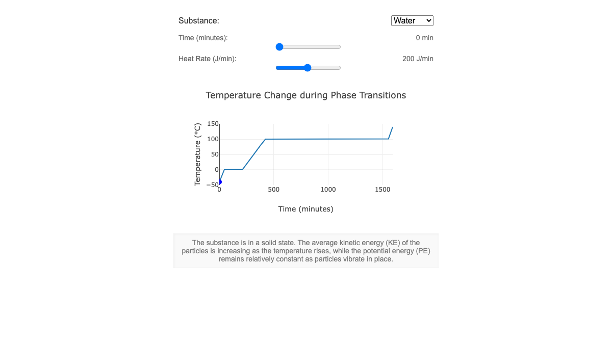
Heating and cooling curves are graphical representations that show how the temperature of a substance changes as heat is added or removed over time. They illustrate the behavior of substances as they go through different states—solid, liquid, and gas.
Heating Curve: This curve shows how the temperature of a substance increases as it absorbs heat. The curve typically rises as the substance heats up, with plateaus indicating phase changes, where the substance absorbs energy but its temperature remains constant. Check out the heating curves for water and nitrogen using the drop-down menu.
Cooling Curve: This curve is the opposite of the heating curve. It shows how the temperature decreases as the substance loses heat. Like the heating curve, it also has plateaus where phase changes occur, but this time, the substance releases energy. In addition to water, you can also see the cooling curve for ethanol.
With these ChatGPT-generated interactive graphs, users can change the rate of heat input or released from the substance. They can also read the descriptions that explain the changes in the average PE and KE of the molecules during each process.
A Geiger-Muller (GM) counter is an instrument for detecting and measuring ionizing radiation. It operates by using a Geiger-Muller tube filled with gas, which becomes ionized when...
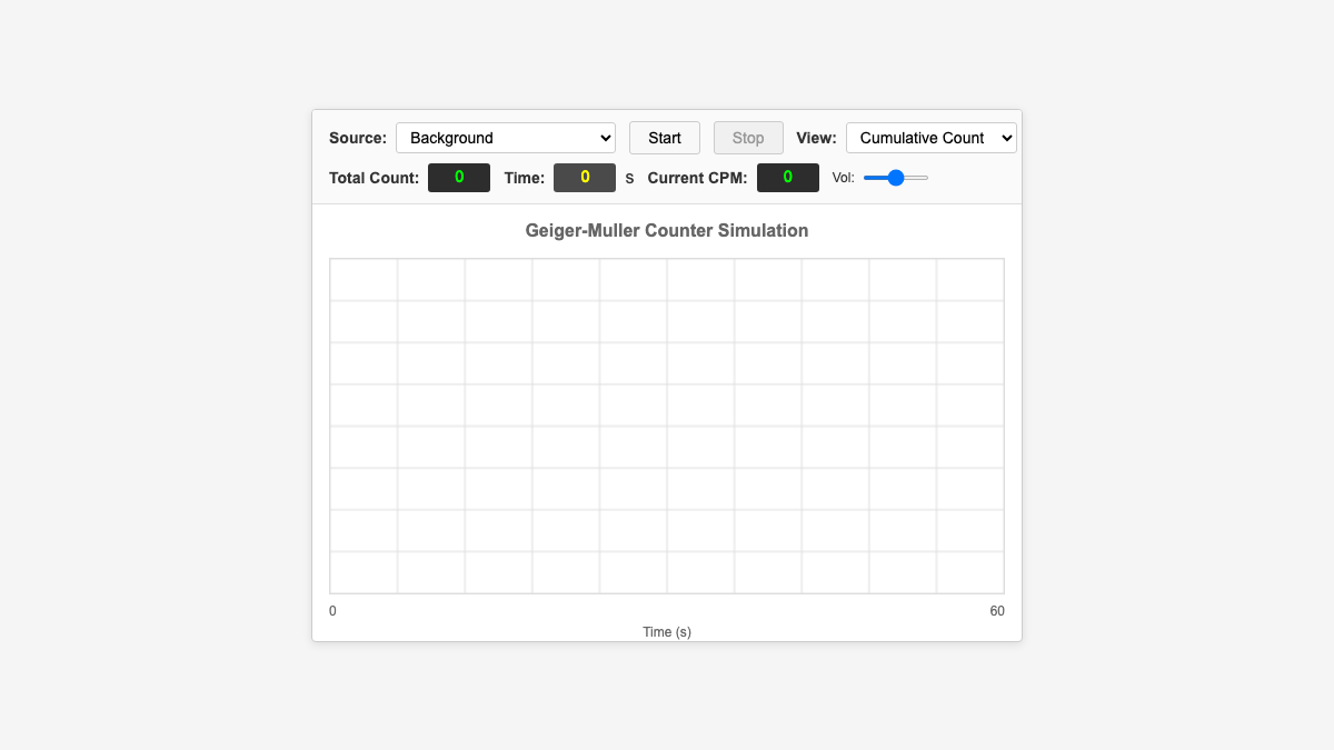
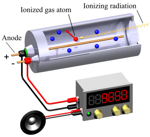
A Geiger-Muller (GM) counter is an instrument for detecting and measuring ionizing radiation. It operates by using a Geiger-Muller tube filled with gas, which becomes ionized when radiation passes through it. This ionization produces an electrical pulse that is counted and displayed, allowing users to determine the presence and intensity of radiation.
This simulation (find it at https://physicstjc.github.io/sls/gm-counter/) allows students to explore the random nature of radiation and the significance of accounting for background radiation in experiments. Here’s a guide to help students investigate these concepts using the simulation.
Exploring Background Radiation
Q1: Set the source to "Background" and start the count. Observe the count for a few minutes. What do you notice about the counts recorded?
A1: The counts recorded are relatively low and vary randomly. This reflects the background radiation which is always present.
Q2: Why is it important to measure background radiation before testing other sources?
A2: Measuring background radiation is important to establish a baseline level of radiation. This helps in accurately identifying and quantifying the additional radiation from other sources.
Investigating a weak source (e.g. banana) as a Radiation Source
Q3: Change the source to "Weak Source " and reset the data. Start the count and observe the readings. How do the counts from the banana compare to the background radiation?
A3: The counts from the weak source are higher than the background radiation. Did you know that bananas contain a small amount of radioactive potassium-40?
Q4: How do the counts per minute (CPM) for the weak source vary over time? Is there a pattern or do the counts appear random?
A4: The counts per minute (CPM) will increase for the first 60 seconds and stabilise slightly after that. The counts per minute for the weak source vary over time and appear random, reflecting the stochastic nature of radioactive decay.
Exploring a strong source, e.g. Cesium-137 Source
Q5: Set the source to "Strong Source" and reset the data. Start the count and observe the readings. How do the counts from the strong source compare to both the background radiation and the weak source?
A5: The counts from the strong source are significantly higher than both the background radiation and the weak source.
Understanding the Random Nature of Radiation
Q6: By looking at the sample counts, can you predict the next count value? Why or why not?
A6: No, you cannot predict the next count value because radioactive decay is a random process. Each decay event is independent of the previous ones.
Q7: How can you use the background radiation measurement to correct the readings from the sources?
A8: You can subtract the average background CPM from the CPM of the sources to get the corrected readings, isolating the radiation from the specific sources.
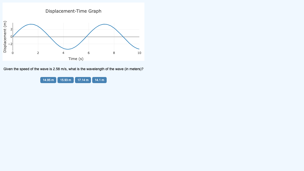
Use the quiz below to test your ability to interpret graphs of waves. You can click on a point in the map to read the values. The codes for this quiz are generated by AI. However,...
Use the quiz below to test your ability to interpret graphs of waves. You can click on a point in the map to read the values.
The codes for this quiz are generated by AI. However, the options and correct answers are rule-based and as such, should not have any errors.
It is able to randomly select from 4 different questions for displacement-distance graphs and 4 others for displacement-time graphs, while randomising the values of amplitude, wavelength and period.
