This simulation offers a clear and interactive way to explore the motion of a ball bouncing on the ground, highlighting how displacement, velocity, and acceleration change over time. On the left, you’ll see the animation of the ball with vectors showing its position (green), velocity (pink), and acceleration (blue). The sliders at the top allow you to adjust the starting height, the percentage of energy lost on each bounce, and whether air resistance is included. You can pause, reset, or let the motion run continuously, while the time slider doubles as a scrubber when the simulation is paused.
On the right, the three graphs display how each physical quantity varies with time. The position–time graph shows the ball’s vertical displacement, always measured relative to the lowest point of its center of mass. The velocity–time graph alternates between negative and positive values, reflecting the downward and upward motion during each bounce, while the acceleration–time graph remains mostly constant at –g, with spikes at the moment of collision. Together, the animation and graphs help link the visual motion with the quantitative data, reinforcing the relationships between these variables.
The underlying theory follows Newton’s laws of motion. The ball accelerates downwards under gravity until it collides with the ground, where it loses some energy depending on the restitution factor. This is why the bounce height diminishes over time. The velocity vector shows not only the speed but also the direction of motion, while the acceleration vector indicates that gravity always acts downward, regardless of whether the ball is rising or falling. By adjusting energy loss during each collision and air resistance, you can model more realistic scenarios and see how dissipative forces affect motion, making this a powerful tool to visualize the physics of bouncing objects.
The above is a GeoGebra applet that can be customised for any energy problem. Simply make a copy of it and change the values or labels as needed. This can be integrated into either GeoGebra Classroom or Google Classroom (as a GeoGebra assignment) and the teacher can then monitor every student’s attempt at interpreting the energy changes in the problem. The teacher can also choose different extents of scaffolding, e.g. provide the initial or final states and ask students to fill in the rest.
What is an LOL Diagram?
An LOL diagram is a tool used to visualize and analyze the conservation of energy in physical systems. “LOL” does not stand for anything meaningful. Rather, they just form the shapes of the two sets of axes and the circle in between. They help clarify which objects or components are included in the energy system being considered and how energy is transferred or transformed within that system.
In LOL diagrams:
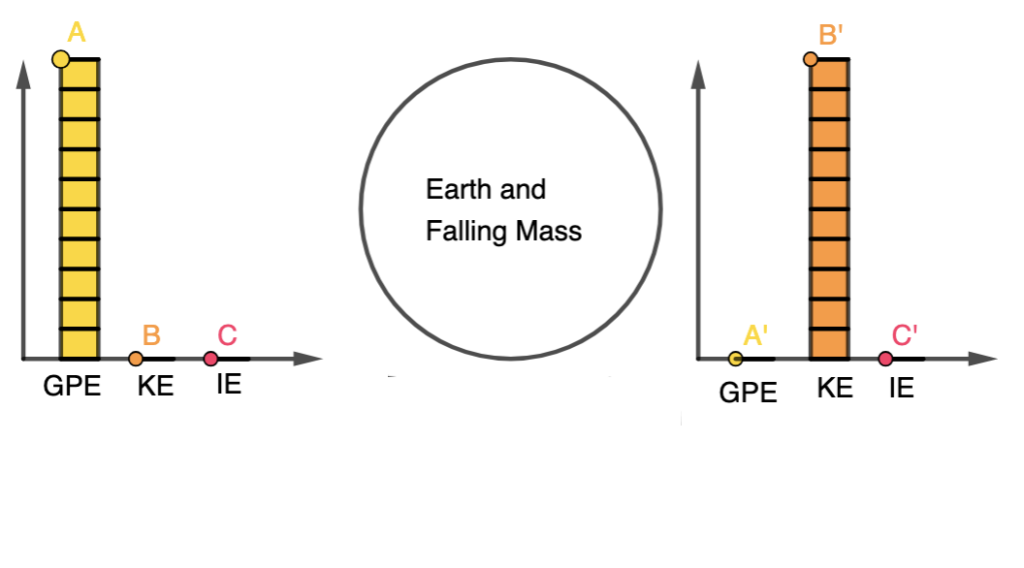
An energy system is defined as an object or a collection of objects whose energies are being tracked.
LOL diagrams consist of three parts: a L-shaped bar-chart representing the initial state, an O representing the object (or system) of interest and another L-shaped bar-chart representing the final state.
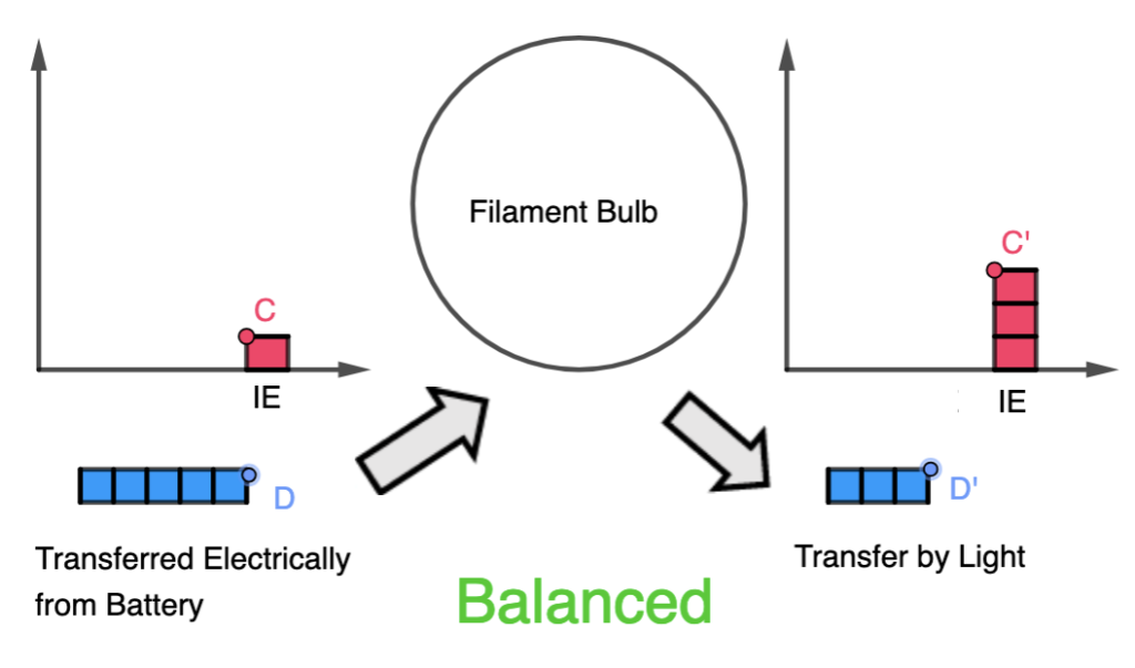
There can also be energy transferred into the system or out of the system if the system is not closed or isolated. These are represented using horizontal bars below the L axes, with arrows indicating if they are energy transferred in or out.
When performing calculations involving the initial and final energy states, the energy transferred into the system is added to the initial energy state while the energy transferred out of the system is added to the final energy state. The sums must be equal. In other words,
Initial energy stores + Energy transferred into system = Final energy stores + Energy transferred out of system
How do I use an LOL diagram?
Here’s a breakdown of how LOL diagrams are used, using an example of a falling mass:
System Definition (O):
Choose what is part of the energy system (objects whose energies are being tracked) and what isn’t.
For example, in the case of a falling mass, the mass itself and the Earth are part of the energy system.
Initial State (L):
Represent the initial energy configuration of the system.
Identify the types of energy present in the system at the beginning. In this example, we begin with some gravitational potential energy.
Transition:
Show how energy changes as the system evolves. In the falling mass example, the gravitational potential energy decreases, and kinetic energy increases.
Final State (L):
Represent the energy distribution in the system at the end of the process.
In the falling mass example, at the point just before it hits the ground, kinetic energy is maximized, and gravitational potential energy is minimized.
LOL diagrams illustrate that energy within the system is conserved, meaning the total energy in the system remains constant.
External work (work done by forces outside the defined system) may impact the system’s energy, but internal work (work done within the defined system) does not change the total energy of the system.
The mathematical representation of the above problem will then simply be:
GPE = KE
$mgh = \dfrac{1}{2}mv^2$
This problem seems a bit trivial. Since LOL diagrams are a visual tool to help students and scientists analyze energy transformations and conservation, they can be used for making it easier to set up and solve conservation of energy equations in problems of greater complexity.
LOL Diagram of an Electrical Circuit
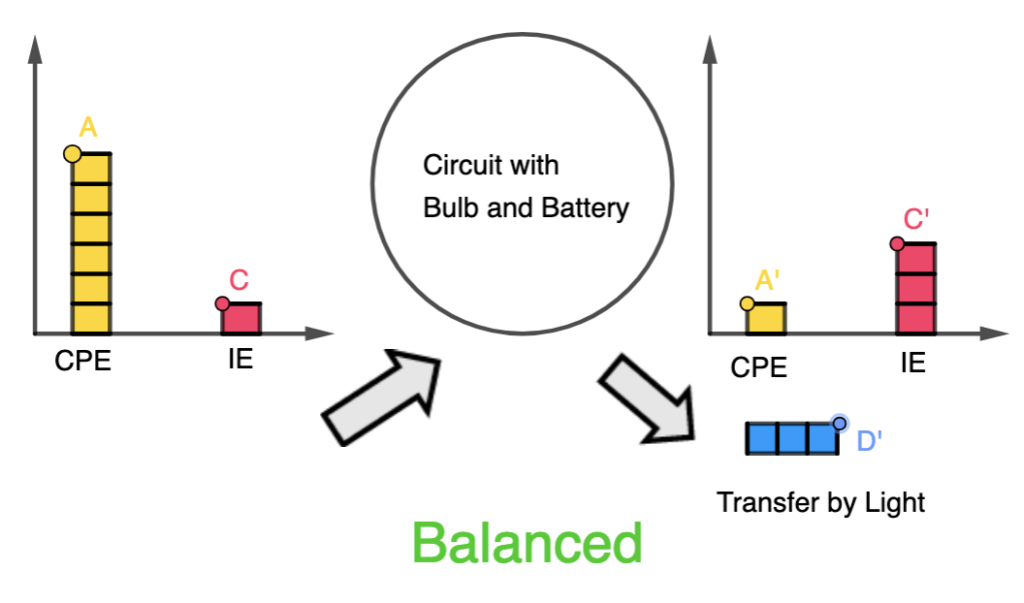
It is also important to note that the choice of the object (or system) of interest will result in different LOL diagrams for the same phenomenon.
For example, consider a filament bulb in a circuit with a battery. The system at room temperature also has some energy in the internal store (or internal energy, which consists of the kinetic and potential energies of the particles in the system).
When considering the filament as the object of interest, when energy is transferred electrically from the battery, part of it is transferred by light from the bulb to the surroundings and another part is added to the internal store, as it heats up the filament light.
On the other hand, when considering the circuit as the whole, the chemical potential store of the battery is included in the initial energy state of the system. Hence, there is no additional energy transfer into the system but the energy transfer output is still the same.
How do I modify the GeoGebra applet to make my own LOL Diagram?
Here’s a video that demonstrates how the editing process is done, in a little more than one minute!
This is the best video I have come across so far that is used to introduce the idea of perpetual motion engines and why it violates the principle of conservation of energy.
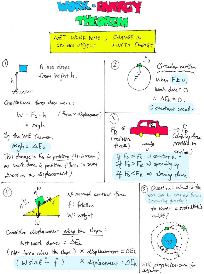
This GeoGebra app allows users to change the magnitude and direction of the force acting on an object, as well as the initial velocity.
The change in kinetic energy is calculated along with the work done in the direction of the force.
This demonstrates a very important concept in Physics known as the Work-Energy Theorem, where the net work done on a particle equals to its change in kinetic energy.