03 Motion and Forces

Kinematics Graphs with Variable Initial Velocity and Acceleration

I used ChatGPT to create this simple interactive graph. Including the time taken to make 2 rounds of refinement using more prompts and the time it took to deploy it via Github, it took about 15 minutes from start to end.

The first prompt I used was :

Create a graph using chart.js with vertical axis being “displacement / m” and horizontal axis being “time / s”. There should be a slider for the initial velocity value ranging from 0 to 2 m/s, a slider for the acceleration value ranging from -2 m/s^2 to 2 m/s^2. The displacement will start from zero and will follow a function dependent on the initial velocity and acceleration values from the slider. Draw the line of the displacement on the graph. Update the graph whenever the sliders are moved.

The results of the first attempt is shown above. It is already functional, with the initial velocity and acceleration sliders working together to change the shape of the graph.

The function it used to calculate displacement is based on the kinematics equation $s = ut + \dfrac{1}{2}at^2$, written as

    displacement.push(0.5 * acceleration * t * t + initialVelocity * t);

After the first successful attempt, I gave some refinement prompts like:

Show the values of the velocity and acceleration, along with the units.

Use drop-down list to change the vertical axis to velocity or acceleration, updating the axis each time and the curve as well.

So the second attempt looked like this

ChatGPT got 1 out of 2 requests correct. The values of the velocity and acceleration were intended to be displayed next to the sliders. It must have been because I was not clear enough. Hence, the last refinement I asked for was :

Give the codes to show the values of velocity and acceleration next to the sliders. Just those codes.

I didn’t want to get ChatGPT to generate the entire page of html and javascript again so I targetted the specific codes that I needed to change.

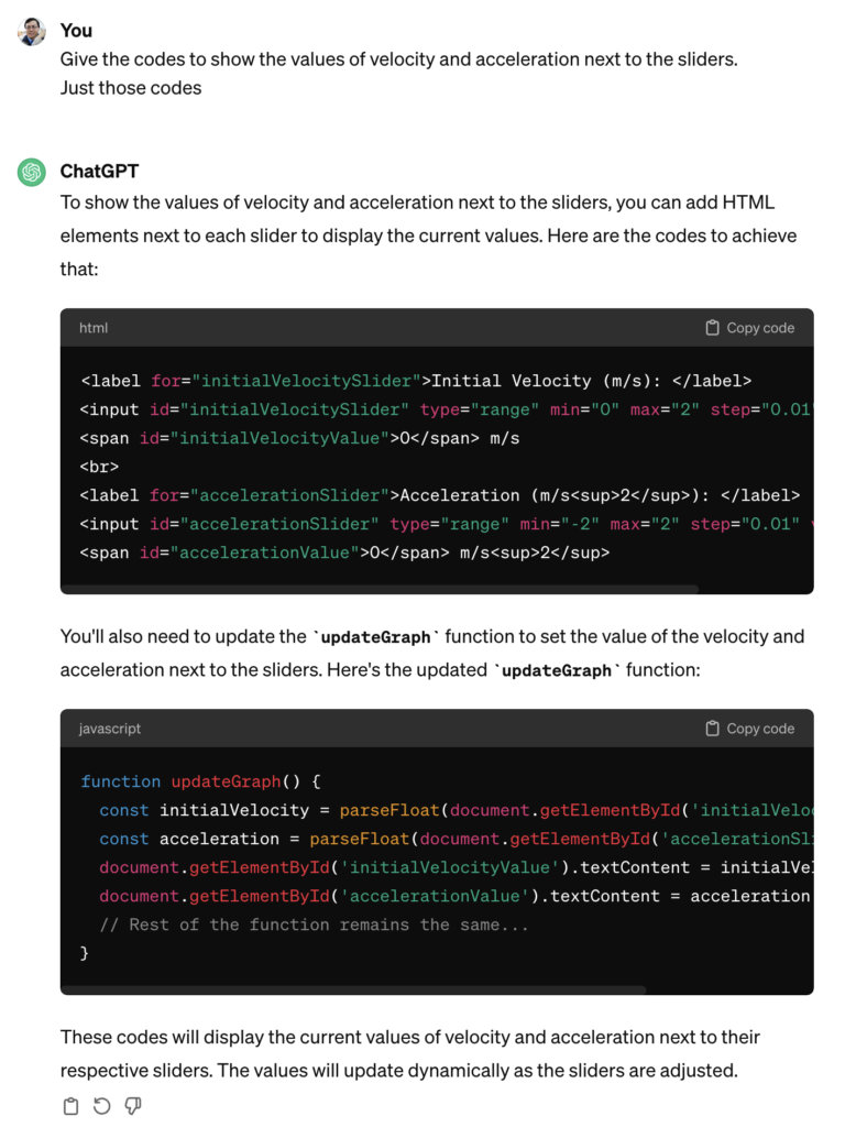
It was helpful in telling me where to update these codes. So at the end of the day, this is what was obtained after I made some manual tweaks to change the way the unit is displayed (e.g. m s-2 instead of m/s2):

It was good enough for my purpose now. The web app can be sent to students as a link (https://physicstjc.github.io/sls/kinematics-graph) or embedded into SLS as a standalone app. For use in SLS, do note the following:

  1. The html file must be named index.html
  2. The chart.js file must be copied and saved in the same zipped file at the same level as the index.html file. Change the path of the Chart JS from <script src=”https://cdnjs.cloudflare.com/ajax/libs/Chart.js/3.7.0/chart.min.js”></script> to <script src=”chart.min.js”></script>.
  3. For reference, this is what it looks like when zipped.

Simulation of a Bouncing Ball

While I have shared a simulation of a bouncing ball made using Glowscript before, I felt that one made using GeoGebra is necessary for a more comprehensive library.

It took a while due to the need to adjust the equations used based on the position of the graphs, but here it is: https://www.geogebra.org/m/dfb53dps

The kinematics of a bouncing ball can be explained by considering the dynamics and forces involved in its motion. In this simulation, air resistance is assumed negligible. When a ball is dropped from a certain height and bounces off the ground, several key principles of physics come into play. Let’s break down the process step by step:

Free Fall: When the ball is released, it enters a state of free fall. During free fall, the only force acting on the ball is gravity. This force is directed downward and can be described by W = mg

W is the gravitational force.
m is the mass of the ball.
g is the acceleration due to gravity (approximately 9.81 m/s² near the surface of the Earth).

Impact with the Ground and Bounce: When the ball reaches the ground, it experiences a force due to the collision with the surface. This force is an example of a contact force and much larger than the gravitational force. This force depends on the elasticity of the ball and the surface it bounces off.

During the collision with the ground, the ball’s momentum changes rapidly. If the ball and the ground are both ideal elastic materials, the ball will bounce back with the same speed it had just before impact. In reality, some energy is lost during the collision, causing the bounce to be less than perfectly elastic. This simulation assumes elastic collisions.

Post-Bounce Motion: After the bounce, the ball starts moving upward. Gravity acts on it as it ascends, decelerating its motion until it reaches its peak height.

Second Descent: The ball then starts descending again, experiencing the force of gravity pulling it back down towards the ground.

This process continues with each bounce. In practice, with each bounce, some energy is lost due to the non-ideal nature of the collision and other dissipative forces like air resistance. As a result, each bounce is typically lower than the previous one until the ball eventually comes to rest. However, for simplicity, the simulation assumes no energy is lost during the collision and to dissipative forces.

An animated gif file is included here for use in powerpoint slides:

Use of System Schema to Visualise Action-Reaction Pairs

It is a common misconception for students to assume that when a book is placed on a table, its weight and the normal contact force acting on it are action-reaction pairs because they are equal in magnitude and opposite in direction.

While we can emphasise the other requirements for action-reaction pairs – that they must act on two different bodies and be of the same type of force – I have tried a different approach to prevent this misconception from taking root. After reading this article on the use of the system schema representational tool to promote understanding of Newton’s third law, I tried it out with my IP3 students.

The system schema identifies the bodies in a question and represents them with shapes detached from each other to give space to draw the connecting arrows between them. The arrows must be labelled with the type of force, either by coding them (e.g. r for reaction force, g for gravitational force) or in full.

Every force will be drawn as a double-headed arrow between two bodies to represent that they are action-reaction pairs. It is important for students to understand that every force in the universe comes in such a pair, and the system schema can help them visualise that. If there is a force without a partner, it just means the system is not in the frame yet.

The next step to using the system schema is for students to isolate the object in question and draw its free-body diagram. Each force vector in the diagram should be accompanied by a name that includes: 1. the type of force and 2. the subject which exerts that force on the object.

The effectiveness of this method of instruction is clearly presented in the paper mentioned above, as performance on the force concept inventory’s questions on the third law saw an improved average from 2.8 ± 1.2 to 3.7 ± 0.8.

Displacement-time graph with animation

This displacement-time graph is used in conjunction with an SLS package to help students learn how to describe motion of an object and to use gradient of a tangent to calculate the magnitude of velocity.

For a direct link to the app, go to https://www.geogebra.org/m/k3ja7bnm

I added a little spider to help students visualise the movement with time.

Man in Elevator

I just took the elevator in my apartment building with the PhyPhox mobile app and recorded the acceleration in the z-direction as the lift went down and up. This was done in the middle of the night to reduce the chances of my neighbours getting into the elevator along the way and disrupting this experiment, and more importantly, thinking I was crazy. The YouTube video below is the result of this impromptu experiment and I intend to use it in class tomorrow.

I used to do this experiment with a weighing scale, and a datalogger, but with smartphone apps being able to demonstrate the same phenomenon, it was worth a try.

To complement the activity, I will be using this simulation as well. Best viewed in original format: https://ejss.s3.ap-southeast-1.amazonaws.com/elevator_Simulation.xhtml, this simulation done in 2016 was used to connect the changes in acceleration and velocity to the changes in normal contact force as an elevator makes its way up or down a building.

Sky-Diving and Terminal Velocity

https://www.geogebra.org/m/wavar9bx

This is a wonderful applet created by Abdul Latiff, another Physics teacher from Singapore, on how air resistance varies during a sky-dive with a parachute. It clearly demonstrates how two different values of terminal velocity can be achieved during the dive.

Incidentally, there is a video on Youtube that complements the applet very well. I have changed the default values of the terminal velocities to match those of the video below for consistency.

Also relevant is the following javascript simulation that I made in 2016 which can show the changes in displacement, velocity and acceleration throughout the drop.