IP3 03 Dynamics

Misconception: Skydiver goes up when parachute opens

When a parachute opens, many people think the parachutist suddenly shoots upward. This is not what really happens. The parachutist is always moving downward, but the parachute causes a very sharp deceleration. The large canopy produces a big upward drag force that slows the fall dramatically.

When people see videos of parachutists opening their parachutes, the camera angle can create a powerful illusion that the parachutist suddenly shoots upward. What really happens is that the parachutist decelerates sharply while the camera, usually attached to another skydiver, continues falling at almost the same high speed.

From the perspective of the camera, the parachutist with the open parachute is no longer keeping pace in the fall. The camera-holder is still dropping rapidly, but the parachutist has slowed down. In the video, this relative motion makes it look like the parachutist has bounced upward, when in fact they are still moving downward—just not as quickly.

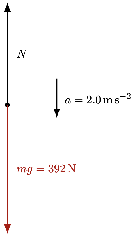
The physics of air resistance shows clearly why the velocity cannot turn upward. Air resistance always acts opposite to the velocity and its size depends on speed. Before and after the parachute opens, the parachutist’s velocity is downward, so the drag force must be upward. If the parachutist’s velocity really were upward, then the drag would have to point downward. In that case, the resultant force would also point downward, making the acceleration greater than gravity—something we never observe. Instead, the drag force remains upward, which proves the parachutist is still moving downward the whole time. The chute simply reduces that downward speed to a safe value.

For a simulation on how the forces and velocity change with time, refer to this GeoGebra app.

A dynamics problem – apparent weight

This is a problem posed by a student today:

A boy of mass 40 kg is standing on a weighing machine inside a lift which is moving upwards. At a certain moment, the speed of the lift is $3.0 \text{ m s}^{-1}$ and it is decelerating at $2.0 \text{ m s}^{-2}$. What is the reading (in kg) shown on the weighing scale?

My advice for any dynamics problem is to take the direction of acceleration as positive. This way, you can apply Newton’s second law directly without worrying about inserting extra negative signs for deceleration. After all, a negative value of acceleration simply comes from the chosen sign convention—it reflects direction. For simplicity, putting the direction of acceleration as positive (in this case, downward is positive), we have

$$F_{net} = ma$$

The net force should therefore, be $W – N$, where $N$ is smaller than $W$.

$$W – N = ma$$

Substituting, we have

$$mg – N = ma$$

$$(40 \text{ kg} \times 9.81 \text{ N kg}^{-1}) – N = 40 \text{ kg} \times 2.0 \text{ m s}^{-2}$$

$$N = 312 \text{ N}$$

Note that $N$ is also known as apparent weight.

The mass reading due to this normal force = $\dfrac{312\text{ N}}{9.81 \text{ N kg}^{-1}} = 32 \text{ kg}$

(Notice here that the speed of the lift is irrelevant.)

The GeoGebra simulation allows you to modify the acceleration and observe the change in the vector representing the normal contact force, which is force acting on the weighing scale.

Open in new tab đź”—

For a real-life experiment along with a visualisation of the changes in the vectors based on this scenario, check out my video and simulation.

Bouncing ball with energy loss

Open in new tab đź”—

This simulation offers a clear and interactive way to explore the motion of a ball bouncing on the ground, highlighting how displacement, velocity, and acceleration change over time. On the left, you’ll see the animation of the ball with vectors showing its position (green), velocity (pink), and acceleration (blue). The sliders at the top allow you to adjust the starting height, the percentage of energy lost on each bounce, and whether air resistance is included. You can pause, reset, or let the motion run continuously, while the time slider doubles as a scrubber when the simulation is paused.

On the right, the three graphs display how each physical quantity varies with time. The position–time graph shows the ball’s vertical displacement, always measured relative to the lowest point of its center of mass. The velocity–time graph alternates between negative and positive values, reflecting the downward and upward motion during each bounce, while the acceleration–time graph remains mostly constant at –g, with spikes at the moment of collision. Together, the animation and graphs help link the visual motion with the quantitative data, reinforcing the relationships between these variables.

The underlying theory follows Newton’s laws of motion. The ball accelerates downwards under gravity until it collides with the ground, where it loses some energy depending on the restitution factor. This is why the bounce height diminishes over time. The velocity vector shows not only the speed but also the direction of motion, while the acceleration vector indicates that gravity always acts downward, regardless of whether the ball is rising or falling. By adjusting energy loss during each collision and air resistance, you can model more realistic scenarios and see how dissipative forces affect motion, making this a powerful tool to visualize the physics of bouncing objects.

Simulation of Projectile Motion with Air Resistance

Open in new tab đź”— This simulation offers a hands-on and dynamic way to explore the physics of projectile motion with and without air resistance. By adjusting parameters such as launch velocity, angle, and air resistance, users can visualize how these factors affect the shape and reach of a projectile’s trajectory. The app provides real-time changes including motion paths, velocity vectors, and a velocity-time graph showing horizontal and vertical components separately. It also calculates and displays key quantities such as maximum height and range under ideal and non-ideal conditions (based on an arbitrary coefficient of drag. Through interactive experimentation and visual reinforcement, learners gain a deeper understanding of concepts the effect of air resistance, and the difference between theoretical and real-world motion. This is suitable for JC1’s topic on projectile motion. It can also be used for Upper Sec, if you change the launch angle to 90 degrees.

Interactive System Schema Generator

I built this web app to help students draw system schemas, having blogged about this before.

It is also available and optimised for download for SLS.

Basic Instructions

To add Bodies:

  • Click the “Add Body” button.​
  • Click on the canvas to place the body at your desired location.​
  • Label the Body.

Add Forces:

  • Click the “Add Force” button.​
  • Click on two bodies that exert the force on each other.​
  • Label the Force.

Using System Schema to Understand Newton’s Third Law

Newton’s Third Law states that when Body A exerts a force on Body B, Body B exerts an equal and opposite force on Body A. While this principle is conceptually simple, many students struggle to apply it consistently across different physical scenarios. The System Schema approach provides a powerful way to visualise and analyse these interactions. It is a representation tool developed by The Modeling Instruction program at Arizona State University (Hinrichs, 2004).

A system schema is a diagram that represents objects (as circles) and interactions (as lines) between them. Instead of focusing on individual forces, a system schema helps students see the relationships between objects before applying force diagrams. This method emphasizes Newton’s Third Law by explicitly showing how forces come in pairs between interacting objects.

To correctly identify action-reaction force pairs, consider the following guidelines:​

  1. Forces Act on Different Objects: Each force in the pair acts on a different object. For example, if Body A exerts a force on Body B, then Body B simultaneously exerts an equal and opposite force on Body A.​
  2. Forces Are Equal in Magnitude and Opposite in Direction: The magnitudes of the two forces are identical, but their directions are opposite.​
  3. Forces Are of the Same Type: Both forces in the pair are of the same nature, such as gravitational, electromagnetic, or contact forces.

The steps to applying System Schema to Newton’s Third Law are as follow:

  1. Identify the bodies in the system – Draw each object as a separate circle.
  2. Represent interactions – Draw lines between bodies to indicate forces they exert on each other (e.g., a box on the ground interacts with Earth through gravitational force).
  3. Label force pairs – Each interaction represents an action-reaction force pair (e.g., a hand pushes a wall; the wall pushes back).
  4. By mapping forces this way, students can easily recognize that forces always act between bodies and in pairs, reinforcing the symmetry of Newton’s Third Law.

One of the most common misconceptions of students is that normal contact force and gravitational force acting on a body are action-reaction pairs because they are equal and opposite in a non-accelerating system. By using the system schema, they can see that the two forces involve interaction with different bodies, e.g. the floor of an elevator for normal contact force, and the Earth for gravitational force.

Use of System Schema to Visualise Action-Reaction Pairs

It is a common misconception for students to assume that when a book is placed on a table, its weight and the normal contact force acting on it are action-reaction pairs because they are equal in magnitude and opposite in direction.

While we can emphasise the other requirements for action-reaction pairs – that they must act on two different bodies and be of the same type of force – I have tried a different approach to prevent this misconception from taking root. After reading this article on the use of the system schema representational tool to promote understanding of Newton’s third law, I tried it out with my IP3 students.

The system schema identifies the bodies in a question and represents them with shapes detached from each other to give space to draw the connecting arrows between them. The arrows must be labelled with the type of force, either by coding them (e.g. r for reaction force, g for gravitational force) or in full.

Every force will be drawn as a double-headed arrow between two bodies to represent that they are action-reaction pairs. It is important for students to understand that every force in the universe comes in such a pair, and the system schema can help them visualise that. If there is a force without a partner, it just means the system is not in the frame yet.

The next step to using the system schema is for students to isolate the object in question and draw its free-body diagram. Each force vector in the diagram should be accompanied by a name that includes: 1. the type of force and 2. the subject which exerts that force on the object.

The effectiveness of this method of instruction is clearly presented in the paper mentioned above, as performance on the force concept inventory’s questions on the third law saw an improved average from 2.8 ± 1.2 to 3.7 ± 0.8.