IP Topics

Use of System Schema to Visualise Action-Reaction Pairs

It is a common misconception for students to assume that when a book is placed on a table, its weight and the normal contact force acting on it are action-reaction pairs because they are equal in magnitude and opposite in direction.

While we can emphasise the other requirements for action-reaction pairs – that they must act on two different bodies and be of the same type of force – I have tried a different approach to prevent this misconception from taking root. After reading this article on the use of the system schema representational tool to promote understanding of Newton’s third law, I tried it out with my IP3 students.

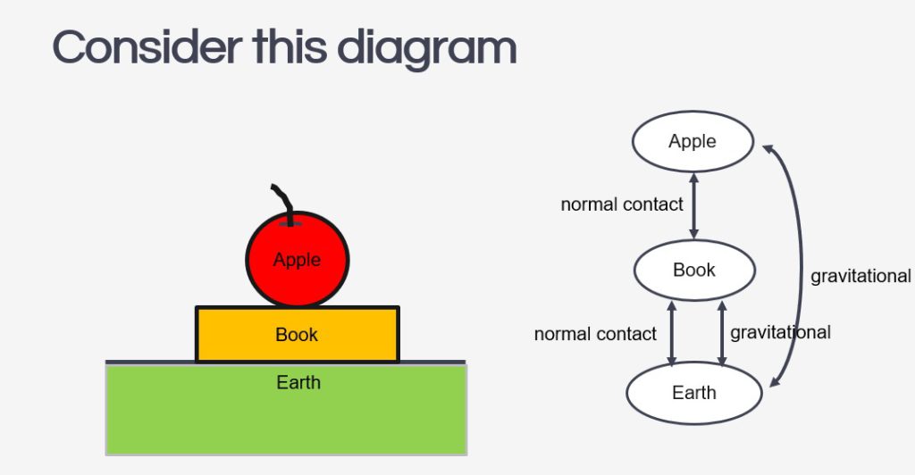
The system schema identifies the bodies in a question and represents them with shapes detached from each other to give space to draw the connecting arrows between them. The arrows must be labelled with the type of force, either by coding them (e.g. r for reaction force, g for gravitational force) or in full.

Every force will be drawn as a double-headed arrow between two bodies to represent that they are action-reaction pairs. It is important for students to understand that every force in the universe comes in such a pair, and the system schema can help them visualise that. If there is a force without a partner, it just means the system is not in the frame yet.

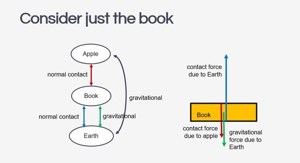
The next step to using the system schema is for students to isolate the object in question and draw its free-body diagram. Each force vector in the diagram should be accompanied by a name that includes: 1. the type of force and 2. the subject which exerts that force on the object.

The effectiveness of this method of instruction is clearly presented in the paper mentioned above, as performance on the force concept inventory’s questions on the third law saw an improved average from 2.8 ± 1.2 to 3.7 ± 0.8.

Vector Addition

I made some refinement to an applet created last year to demonstrate how vector addition can be done either using vector triangle or parallelogram methods.

To access directly in Geogebra, the link is https://www.geogebra.org/m/p2yvdsvs

Unit Conversion Self-Practice

This new applet is designed for students to practise conversion of common units used in physics on their own. There is a checking algorithm within, which might need some fine-tuning. For full screen view, click here.

The worked solutions given will demonstrate the breakdown of steps that could help students learn the procedure to convert these units.

Standard Form and Prefixes

This little applet is designed to allow students to change the order of magnitude and to use any common prefix to observe how the physical quantities are being written. To view this applet in a new tab, click here.

Standard form (also known as scientific notation) is a way of writing very large or very small numbers that allows for easy comparison of their magnitude by using the powers of ten. Any number that can be expressed as a number, between 1 and 10, multiplied by a power of 10, is said to be in standard form.

For instance, the speed of light in vacuum can be written as 3.00 × 10⁸ m s–1 in standard form.

When a prefix is added to a unit, the unit is multiplied by a numerical value represented by the prefix. e.g.     distance = 180 cm = 180 x 10-2 m = 1.80 m

The purpose of using prefixes is to reduce the number of digits used in the expression of values. Hence, students can use the prefix slider to find a user-friendly expression, such as 682 nm instead of 0.000000682 m.

The ten prefixes used are:

10-12pico
10-9nano
10-6micro
10-3milli
10-2centi
10-1deci
103kilo
106mega
109giga
1012tera

Hidden Dangers Of Water Heater: How To Install It Safely?

This rather informative video uses a recent local case of electrocution as a case study and goes on to explain various practical electricity concepts such as electric faults (e.g. live wire connected to earth wire). Recommended for students learning about O-level Practical Electricity, although I would caution them that some of the dialogue is based on a layman’s understanding of how electricity works, so there are some scientific inaccuracies.

Appreciating the least square method of determining best-fit line

This interactive is designed to help students understand the statistical approach underpinning the drawing of a best-fit line for practical work. For context, our national exams have a practical component where students will need to plot their data, often following a linear trend, on graph paper and to draw a best-fit line to determine the gradient and y-intercept.

The instructions to students on how to draw the best-fit line is often procedural without helping students understand the principles behind it. For instance, students are often told to minimise and balance the separation of plots from the best-fit line. However, if there are one or two points that are further from the rest from the best-fit line (but not quite anomalous points that need to be disregarded), students would often neglect that point in an attempt to bring the best fit line as close to the remaining points as possible. This results in a drastic increase in the variance as the differences are squared in order to calculate the “the smallest sum of squares of errors”.

This applet allows students to visualise the changes in the squares, along with the numerical representation of the sum of squares in order to practise “drawing” the best-fit line using a pair of movable dots. A check on how well they have “drawn” the line can be through a comparison with the actual one.

Students can also rearrange the 6 data points to fit any distribution that they have seen before, or teachers can copy and modify the applet in order to provide multiple examples of distribution of points.